Error Analysis and Least Squares Fitting
 

Equipment used:

1) Index cards
2) Grog strip
3) Spreadsheet

Objectives:

A) Provide a brief overview of statistical error analysis and propagation of errors.

References:

John R. Taylor, An Introduction to Error Analysis, Second Edition, University Science Books, Sausalito, California (1996).
D. W. Preston and E. R. Dietz, The Art of Experimental Physics, John Wiley & Sons, New York (1991); pp. 7-28.
C. Cooke, An Introduction to Experimental Physics, University College London Press, London (1996); Chapter 5, pp. 65-101.
S. L. Meyer, Data Analysis for Scientists and Engineers, John Wiley & Sons, New York (1975).
 

Whenever you perform an experiment or measure a quantity with a suitable measuring device the question arises: How reliable is the result? How close does the result come to the real value – whatever that may be?

It is easy to say how close to the real value you are – how accurate the measurement is – if you know what the real value is. For instance, if you measure the temperature of a glass of pure water with floating ice cubes (at a pressure of 1 atmosphere) your thermometer might indicate a temperature of -1^oC (or 30^oF). However, you know that the temperature of water under those conditions would be 0^oC (or 32^oF), thus it is clear that your measurement is "off" by 1^oC. There could be a number of reasons why the result is off in this example: the thermometer’s calibration is not very good, you might look at the scale at an angle (parallax), environmental conditions might be wrong, e.g. pressure different from 1 atmosphere, or the water might contain impurities. All these conditions would cause an error in your result, however, this error is systematically tied to the problem, i.e., the error can be reproduced. This type of error is called systematic error, and these errors can be identified and, in principle, eliminated. If a measurement has small systematic errors, it is said to have high accuracy.

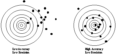
Often you do not know what the real value of the measured quantity is. If the measurement is repeated a number of times you might find that the result is a little different each time, however, not in a systematic or predictable way. These variations in the result are due to random or statistical errors. Often the sources of random errors cannot be identified, and random errors cannot be predicted. Thus it is necessary to quantify random errors by means of statistical analysis. Simply by repeating an experiment or a measurement several times you will get an idea of how much the results vary form one measurement to the other. If there is little variation of the results you have a high precision, whereas large variations in the result indicate low precision. A way to visualize accuracy and precision is by the example of a dart board. If you are a poor "dartist" your shots may be all over the board – and the wall; each shot hitting quite some distance from the other: both your accuracy (i.e. how close you are to the bull’s eye) and your precision (i.e. the scatter of you shots) are low (below left).

If you are somewhat better, you will at least consistently hit the board, but still with a wide scatter: now your accuracy is high, but the precision remains low (above right). Once you get consistent and there is not much scatter in your shots, your results may look like this:

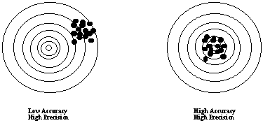
Above left is not very accurate, however, your shots have high precision; once you work out this systematic "drift to the right" your shots will be very accurate and very precise (above right) and you may be ready to challenge the champion.

What should be used to quantify the random error of a measurement? If only a single measurement y is made, you must decide how closely you can estimate the digit beyond those which can be read directly, perhaps 0.2 to 0.5 of the distance between the finest divisions on the measuring instrument. However if a set of N measurements is performed it is proper to quote, as the result of the measurement, the mean value or average value:

Here the yi are the results of the N individual measurements. The errors in measurement of y are assumed to follow a Gaussian or normal distribution, the familiar "bell-shaped curve". The standard deviation is used to describe the spread or precision of a set of measurements. Suppose the standard deviation of that theoretical distribution is s. If one more measurement of y is made, there is 68% probability that the result will fall within . Let s be the best estimate of s; it is obtained from your N measurements as

Note that s is not quite equal to the root-mean-square deviation of the N measurements. The N-1 instead of N in the denominator results from the fact that at least two measurements must be performed in order to specify the standard deviation.

Instinctively we expect that if more measurements of y are made, the uncertainty in the result ought to get smaller. Again assuming the errors in measurement of y follow a Gaussian distribution, the standard deviation of the mean of N measurements turns out to be . This means that if the whole set of N measurements is repeated, there is a 68% probability that the mean value of the new set of measurements will be within . The best estimate of this quantity from your N measurements is

In summary, when quoting the result of N measurements of a quantity y, you should quote the result as

Outright blunders such as misreading measuring instruments or making arithmetic errors in processing the data have no place in a well-done experiment. Unlike random errors, blunders can be eliminated completely.

Error does not mean discrepancy between your result and the "right" result found in some textbook. Some day you will probably be the first person ever to measure some physical quantity, and then there will be no other result with which to compare yours. Yet it is still your responsibility to estimate the amount of error or uncertainty in your result, to indicate your level of confidence in your measurement. And this responsibility goes on and on with every measurement you make, through PHY 293 and into the future. It is kind of like filling out your income tax return: just because you did it on one occasion does not mean you do not have to do it again! The following exercises are designed to practice some of the error analysis procedures your are likely to encounter during this course.

1. Spreadsheet

Turn on your computer and run your spreadsheet program, by double-clicking on the icon on the Windows desktop. Then set up a spreadsheet consisting of four columns. The first column contains the index i running form 1 to 10. The second column has some data value x(i), which could be the result of a measurement performed 10 times (N = 10). Note that each value is slightly different from the other. At the bottom of this column calculate the sum of the x(i) and the mean = sum/10. In the next column calculate the simple deviation from the mean, and in the last column the squared deviation of the mean. At the bottom of the last column you can evaluate the sum of the (x(i) - mean)2 and the standard deviation as well as the standard deviation of the mean. When you are done your spreadsheet should look somewhat like this:
 

		i	x(i)	(x(i)-mean)	(x(i)-mean)^2
		1	2.00	#.###	#.######
		2	2.03	#.###	#.######
		3	1.98	#.###	#.######
		4	2.01	#.###	#.######
		5	1.95	#.###	#.######
		6	2.02	#.###	#.######
		7	2.01	#.###	#.######
		8	1.97	#.###	#.######
		9	2.01	#.###	#.######
	N =	10	1.99	#.###	#.######
Sum =			#.##	#.###	#.######
Mean =			#.###
		Standard deviation =			#.###
		Standard dev. of the mean =			#.###

The #.### indicate the digits you should format the corresponding cell to display. You just calculated the mean value, the standard deviation, and the standard deviation of the mean for the given x(i) with N=10 "manually", i.e. without using any spreadsheet function other than the sum. Of course, any self-respecting spreadsheet will have built-in functions for the mean value and the standard deviation. Try and see if you can add these functions to the spreadsheet above to check if they return the same numbers as your own calculation.

2. Measurements

For this exercise you can use your spreadsheet to calculate the same quantities, this time we will actually perform a measurement several times by all students in the lab to get some random error. We will measure the long side of the index card you have at your table using a GROG-strip. The GROG strip is similar to a meter or yard stick, except it has a scale in units of centigrogs (abbreviated as cg). 1cg is approximately 9 mm or 7/8". There are no further divisions, such as milligrogs, so will be forced to estimate the fractions. Every student in the lab should do one measurement and write the result on the black board. When all values are written down, transfer them to your spreadsheet to calculate mean, standard deviation, and standard deviation of the mean. Besides practicing some basic statistical analysis and spreadsheet skills, this example also demonstrates the utility of a spreadsheet. Once set up for a given calculation you can reuse it simply by entering new numbers in the right places. In some of the experiments in this course we will be using pre-made spreadsheet templates to focus on the results of our experiment rather than the process of setting up the spreadsheet. Later in the course you will be required to set up your own spreadsheets.

3. Propagation of Errors

In the example above we have seen how we can quantify the random errors present in a measurement. Suppose we cannot repeat a measurement, or if we repeat it the same way we get the same result (as in one person making repeated measurements with a ruler)? In such cases we try to estimate the error. Whenever the measuring device has a scale, e.g. meter stick, GROG-strip, voltmeter, etc., we can use 1/2 of the smallest scale unit as the estimate of error, the so-called probable error. Thus a single measurement of the index card length with the GROG-strip would be reported as (13.4 ± 0.5) cg.

Assume we now want to determine the area of the index card. For this we have to measure the length and the width and then multiply the values to obtain the area. But since the length and width have an error (or uncertainty), the calculated area will also have an error or uncertainty associated with it as the errors of width and length propagate through the calculation. Suppose the component quantities are independent of each other, i.e. the error in measuring one does not influence the error in measuring the other. Then error in one measurement might tend to make the final result too big, while error in another might affect the final result in the opposite direction. Allowance for the possible cancellation is made by taking the square root of the sum of the squares of the contributions due to the individual measurements.

If the quantity z is a function of independent quantities x and y, we write for the uncertainty in z

Generalization to more than two component measurements is straightforward.

Now measure the length and width of your index card with the GROG-strip, calculate the area and the associated uncertainty. When you are done, write your result on the black board so we can compare it with everyone else’s. Once all the results are on the board calculate the average area and the resulting error. Watch out, this is not the same as the standard deviation of the mean, as there it is assumed that the error in each measurement is the same. In our case the error with each lab team’s result is bound to be slightly different. Hint: use the definition of the propagation of error (the equation above the first of the three examples from above).

4. Least Squares Fitting

Consider a set of data points (x_i, y_i). We would like to fit a curve to these data points. In general there is an experimental uncertainty associated with the values of both x and y. However the curve- fitting problem becomes extremely difficult in this general case. Fortunately, in physics we often encounter situations where values of x are much better determined than values of y. We will consider the case where each xi is assumed to be known exactly, and there is an uncertainty Dy_iassociated with each point (Dy_i usually corresponds to one standard deviation s_i in a set of measurements of y_i).

We are going to consider the case where the data points can be fitted wirh a straight line. As you can see from the figures, uncertainty in the y values leads to considerable uncertainty in what line to draw.

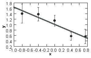
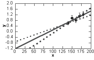
Above left is a plot of data points of unequal weight showing just the range measured.  The best fit line is displayed.  On the right is a plot of data points taken in the range x > 140.  The fitted straight line is extropolated to the point x = 0.  The dotted lines indicate the uncertainties in the determination of slope and intercept.

Again under the assumption that the errors have a normal distribution, the "best fit" or regressionline is obtained by minimizing the sum of the squares of the deviations of the measured y_i’s from the corresponding fitted y_i’s. In doing this sum, each square term is weighted according to the uncertainty of the corresponding y_i. The assigned weight wi is

So in fitting a straight line y = m x + b to N data points, we minimize the sum

with respect to the slope m and the y-intercept b. This leads to the equations

(1) 

(2) 

If we define 

equation (1) reduces to 0 = E - mD - bA and equation (2) gives 0 = C - mA - bB. This pair of equations can be solved for m and b by Cramer’s rule:

With somewhat more difficulty one can derive the errors of the slope m and the intercept b (see Meyer pp. 366-7)

Chi-Square and Goodness of Fit

Once we have our fit, we would like to know "how good" it is. Clearly if many of the data points do not lie on the fitted line, the fit is not very good. Note that if the mean values yi lie off the line but the uncertainties are large enough to overlap the line, the fit is better.

Statisticians have derived a quantitative measure of goodness of fit called the chi-square (c²) test (for example see Taylor, chapter 12). The objective of the test is to assign a probability that if the measurements were repeated, the weighted sum of the squared deviations [y_i - (m x_i + b)]² would be larger, that is, the "miss" of the fit would be more.

For our purposes all you need to know about chi-square is that for a given set of data points, the larger the value of chi-square, the poorer the fit. Computer programs are available to calculate values of chi-square so you can compare "goodness" of your fits.

In closing, a good summary statement is taken from Cliff Swartz in an editorial in The Physics Teacher: