
Jan Yarrison-Rice with Jennifer Malos
Equipment Used:
Convex Lens, HeNe Laser, Air Force Resolution Chart, Iris Diaphragm Aperture, Glass Slide with Spot, CCD Camera, Monitors, and Macintosh Computers with NIH Image Program.
Objectives:
The goal of this laboratory experiment is to familiarize students with basic lens properties, demagnification and magnification of images, and simple spatial filtering.
References:
E. Hecht, Optics, 3rd edition, Addison Wesley Longman, Reading, Massachusetts (1998).
F. Pedrotti, S.J. and L. Pedrotti, Introduction to Optics, Prentice-Hall, Englewood Cliffs, New Jersey (1987).
Light as A Wave:
Fig. 1: Characteristics of a wave
Equation describing relation between wavelength (l),
frequency (f), and speed of light (c).
c = lf
Light exhibits many properties. Some are wave-like and others particle-like. Experiment #1 discussed how light acts as a particle. Here we will explore lights wave nature. As light propagates through space and matter it acts like a wave. These characteristics include interference, diffraction, and refraction as well as reflection.
A description of refraction might be as follows.
When propagating light encounters a dense medium (going from low to high
index of refraction), it slows down. If the light is traveling at an angle
when it strikes the medium, the light is bent as it goes from air into
the denser medium. This bending is called refraction. Light bends toward
the normal line as it enters a higher index material, and away from the
normal line when it enters a less dense (lower index) material. Snell's
Law of Refraction tells us what angle the light will bend through depending
on the input angle and the index of refraction of the two mediums through
which the light travels.
Snells Law:
n1 sin W = n2 sinj
If n1 is less than n2
(as is the case for air and Plexiglas), then W
> j. The index of
refraction of air, n1 = 1.00.
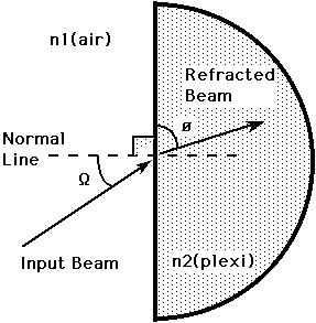
Fig. 2: Illustration of Snells law of refraction
There 2 major lenses that are used to manipulate light - to refract or bend the light and change its direction - a convex lens and a concave lens. You have one of each. A concave lens has concave surfaces (curving inward) which takes incoming light and bends it away from the center of the lens, thus spreading out the light as it passed to the other side of the lens. A convex lens has convex surfaces (bulging outward) which take the incoming light and bends it toward the center of the lens, thus focusing the light into a tight spot on the other side of the lens.
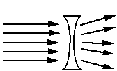
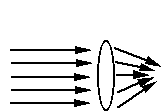
Fig 3a: A biconcave lens
Fig 3b: A biconvex lens
There are a few definitions which describe lenses
and their uses. When light from far away (like from the sun) is bent by
a lens to form a small spot, the distance to that spot is called the focal
length of the lens. The picture created from light reflecting off a nearby
object that strikes a lens and is bent while traveling through to screen
is called an image. Your eyeball is a big lens with detectors behind it.
Q:
What type of lens is your eye?
a) Take your lens and look at print in your booklet.
Q:
What do you see? Q: How does this view change as you move the lens
up and down above the print? Guess which type of lens this is.
b) Try to use the lens to form a focused image of
the light in the ceiling on the lab bench. Record what happens with each
lens. Use light from outside to produce an image and take a ruler to estimate
the lens's focal length.
Imaging with Convex Lenses
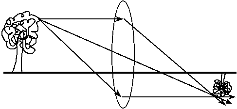
Fig 4: Image of a tree with a converging lens.
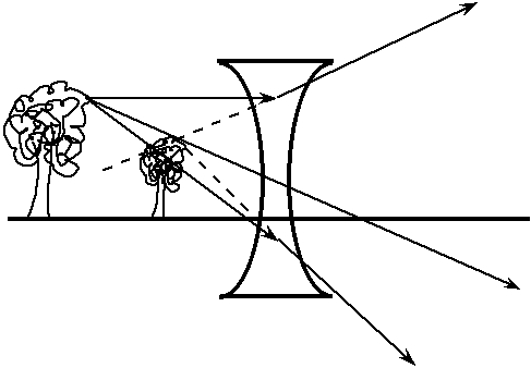
Fig. 5: Image of a tree with a diverging lens.
Let's explore the fundamental imaging equation ![]() where f is the focal length of the lens, o is the object distance from
the lens, and i is the image distance from the lens.
where f is the focal length of the lens, o is the object distance from
the lens, and i is the image distance from the lens.
An optical system is set up in the lab that will pass laser light through the resolution chart, through a lens, and then onto a screen. Draw a diagram of your apparatus including distances, focal lengths and other optics placement.
DO NOT LOOK DIRECTLY INTO THE LASER
BE CAREFUL OF REFLECTIONS
>>>>>>>>>>> YOUR SAFETY IS PARAMOUNT <<<<<<<<<<<<
Vary the distance between lens, chart, and screen and check image.
Q2: Is it upright or inverted?
Create a magnified image and then measure your image magnification using the resolution chart's known spatial frequencies and a ruler. Then calculate the magnification of the image you should have produced for comparison.
Q3: In your present set-up, (i.e. with the resolution chart and convex lens position kept the same), what focal length lens would you require to magnify the image 20 times? and how far should the screen be placed to do so?
Q4: With your lens, could you produce a de-magnified image? How?
Q5: What happens to the image if you block
half the lens? The other half? Can you predict this behavior with a series
of rays going through the lenses. Draw the schematic. (Hint: Are the rays
coming into the lens parallel now?)
Spatial Filtering -- One Form of Image Processing
Spatial filtering is accomplished in the Fourier
Transform plane of a lens. This occurs in the focal plane of the lens.
Light that passes through a lens will form the Fourier Transform of the
spatial information in the beam at the focal plane. This means that the
spatial information is moved into a new pattern in which low frequency
components are near the center of the new beam and higher frequency components
produce spots leading away from the central dot at angles reflecting the
position of the higher spatial frequencies. Mathematically, we can show
that the Fourier Transform of a spatially varying image is equivalent to
the far field diffraction pattern of an aperture that has the same spatial
variation. For instance, 1 vertical line placed in the beam would create
a Fourier Transform with a central dot and several dots decreasing in size
and separation to the right and left on a screen in the focal plane which
is the diffraction pattern of 1 slit placed in a beam.
![]()
Fig. 6: The Fourier transform of a
single slit is the
same as the far field diffraction pattern of a single
slit.
Recall your predictions for the Fourier Transforms of triangles and circles as you do the following exercises.
Spatial filtering terminology is as follows. The term "high or low" frequency filtering means that the filter blocks the specified frequency range and the term "high or low" pass filter means that the specified frequency range is allowed to pass through the filter. For example, low spatial frequency filtering can be used to enhance high spatial frequencies, producing what is called an edge enhanced image in the image plane by blocking low spatial frequencies in the Fourier plane. Whereas a low pass filter produces a blurry image by blocking high frequency components in the Fourier plane and allowing low frequency components to pass.
Computer Simulation of Optical Processing
Lets predict our experimental results by utilizing the software package, Image 1.2. (on the PowerMac Image 1.59) Open Image (double click), Select New under FILE, and a blank screen will come up on the computer [PowerMac choose Width: 512 and Height: 512, Then click on OK]. Use the tool bar to draw an elongated rectangle on the screen that we envision our beam passing through. This can be accomplished with the Tool Bar and then using Fill under EDIT to blacken the inside of the selected portion of the picture. Next choose Select All under EDIT to encircle the pattern and choose FFT (fast Fourier transform) from the FFT bar on the menu [PowerMac go under PROCESS and choose FFT]. After a brief calculation, the FFT will appear on a new screen. Now check to see if it has the high frequency components that you would expect from your drawing (in general).
Then using the tool bar place a spatial filter on the FFT (it can be a low or high pass filter). This allows you to box in certain areas of your FFT with symmetrically placed circles or quadrangles. By choosing Filter (which blocks the inside of selected area) or Pass (which keeps only the information within the selected area) under FFT on menu the filtering is accomplished. [PowerMac users must use Tool Bar to filter with squares or circles and then push Delete button on keyboard to remove selected space and produce filter. Selection of center or edges of FFT produce high or low pass filtering.] Lastly have the computer take the Inverse FFT of the spatially filtered FFT of the image under FFT on menu [or under PROCESSES, then FFT for PowerMac]. The resulting image is what you would expect to observe on the screen in the image plane with the particular type of filter you created.
You can use a box from the Tool Bar to draw a horizontal line through the picture. Under ANALYZE choose Column Average Plot [Plot Profile on PowerMac] to see how clean the edges are before and after spatial filtering.
Next try a triangle to check your prediction for the FFT and then try both types of spatial filters in the simulation.
You also have a file with the resolution chart. Note: The experimental apparatus you have available is an Air Force Resolution Chart. Create high and low frequency filtering of this image. Use the line on plot profile to check profile for edge sharpness before and after filtering.
Q6: What do you note about low versus high frequency filtering? How do the plot profiles look?
Be sure to sketch what each step looks like on the screen.
Experimental Optical Filtering
With the optics and spatial filtering devices available, set-up and explore the following optical filtering systems.
a) Low frequency filtering.
b) High frequency filtering of a single orientation of line (vertical, horizontal, +45 degree).
For Your Report:
1. Draw diagrams of all optical systems while doing experiments.
2. Note results both with words and pictures.
3. Answer questions posed in the experimental description.
In addition, answer the following questions as part
of the conclusion section.
A. With a drawing of a large plano-convex lens and a plano-concave lens, using 3 input rays measure input angles and calculate output angles in each lens. Demonstrate how and where the rays are focused for each case.
B. Describe a contemporary situation in which image processing could be used.
C. What qualities of light did you explore in the last experiment and how do they compare with what you learned in this experiment?
D. How do you reconcile the above differences in experiment 1 and 2? What do the great "modern" physicists say about this dual nature of light?
| This document was last modified on Friday, 01-Sep-2000 18:46:22 EDT
and has been accessed [an error occurred while processing this directive] times. Address
comments or questions to:
|